Deconvolutional Networks for Point-Cloud Vehicle Detection and Tracking in Driving Scenarios
Deconvolutional Networks for Point-Cloud Vehicle Detection and Tracking in Driving Scenarios
Abstract
Vehicle detection and tracking is a core ingredient for developing autonomous driving applications in urban scenarios. Recent image-based Deep Learning (DL) techniques are obtaining breakthrough results in these perceptive tasks. However, DL research has not yet advanced much towards processing 3D point clouds from lidar range-finders. These sensors are very common in autonomous vehicles since, despite not providing as semantically rich information as images, their performance is more robust under harsh weather conditions than vision sensors. In this paper we present a full vehicle detection and tracking system that works with 3D lidar information only. Our detection step uses a Convolutional Neural Network (CNN) that receives as input a featured representation of the 3D information provided by a Velodyne HDL-64 sensor and returns a per-point classification of whether it belongs to a vehicle or not. The segmented point cloud is then geometrically processed to generate observations for a multi-object tracking system implemented via a number of Multi-Hypothesis Extended Kalman Filters (MH-EKF) that estimate the position and velocity of the surrounding vehicles. The system is thoroughly evaluated on the KITTI tracking dataset, and we show the performance boost provided by our CNN-based detector over the standard geometric approach. Our lidar-based approach uses about 4% a fraction of the data needed for an image-based detector with similarly competitive results

Paper Summary

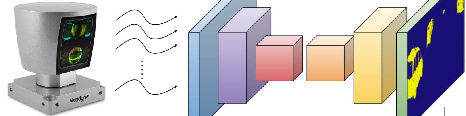
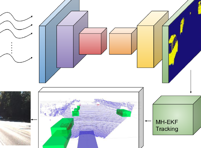
We introduce a novel CNN-based vehicle detector on 3D range data. The proposed model is fed with an encoded representation of the point cloud and computes for each 3D point its probability of belonging to a vehicle. The classified points are then clustered generating trustworthy observations that are fed to our MH-EKF based tracker. Note: Bottom left RGB image is shown here only for visualization purposes.
Lidar Data Representation

To obtain a useful input for our CNN-based vehicle detector, we project the 3D point cloud raw data to a featured image-like representation containing ranges and reflectivity information by means of $G(\cdot)$. In this way, we first project the 3D Cartesian point cloud to spherical coordinates $sph(p_i)~=~{\phi_i,\theta_i, \rho_i}$. According to the Velodyne HDL-64 specifications, elevation angles $\theta$ are represented as a $H \in \mathbb{R}^{64}$ vector with a resolution $\Delta\theta$ of 1⁄3 degrees for the upper laser rays and 1⁄2 degrees the lower half respectively. Moreover, $G(\cdot)$ needs to restrict the azimuth field of view, $\phi \in [-40.5,40.5]$ to avoid the presence of unlabelled vehicle points, as the Kitti tracking benchmark has labels only for the front camera viewed elements. The azimuth resolution was set to a value of $\Delta\phi=0.18$ degrees according to the manufacturer, and hence lying in $W \in \mathbb{R}^{451}$. Each $H,W$ pair encodes the range ($\rho$) and reflectivity of each projected point, so finally our input data representation lies in an image-like space $G(\mathcal{P}) \in \mathbb{R}^{64 \times 451 \times 2}$.
Ground-truth for learning the proposed classification task is obtained by first projecting the image-based Kitti tracklets over the 3D Velodyne information, and then applying again $G(\cdot)$ over the selected points.
Network Used

Our network encompasses only convolutional and deconvolutional blocks followed by Batch Normalization (BN) and ReLu (RL) non-linearities. The first three blocks conduct the feature extraction step controlling, according to our vehicle detection objective, the size of the receptive fields and the feature maps generated. The next three deconvolutional blocks expanse the information enabling the point-wise classification. After each deconvolution, feature maps from the lower part of the network are concatenated (CAT) before applying the normalization and non-linearities, providing richer information and better performance.
During training, three losses are calculated at different network points, as shown in the bottom part of the graph:
$\mathcal{L}(\hat{\mathcal{Y}}, \mathcal{Y})$ = $\sum_{r=1}^{3}$ $\lambda_r \mathcal{L}_r (\hat{\mathcal{Y}_r}, {\mathcal{Y}_r})$ ,
where $r$ represents the intermediate loss-control positions, $\lambda_{r}$ are regularization weights for the loss at each resolution, and $\hat{\mathcal{Y}}, \mathcal{Y}$ are respectively the predictions and ground-truth classes at those resolutions.
In our approach, $\mathcal{L}_r$ is a multi-class Weighted Cross Entropy loss (WCE) defined as:
$\mathcal{L}_r^{WCE}$ = $-\sum_{i,j,k}^{H_r,W_r,K_r}$ $\omega(\mathcal{Y}_{i,j})$ $\textit{Id}_{[\mathcal{Y}_{i,j}]}$ $\text{log}(\hat{\mathcal{Y}}_{i,j,k})$ ,
where $\textit{Id}_{[x’]}(x)$ is an index function that selects the probability associated to the expected ground truth class and $\omega(k)$ is the previously mentioned class-imbalance regularization weight computed from the training set statistics.
Results


Acknowledgements: This work has been supported by the Spanish Ministry of Economy and Competitiveness projects ROBINSTRUCT (TIN2014-58178-R) and COL- ROBTRANSP (DPI2016-78957-R), by the Spanish Ministry of Education FPU grant (FPU15/04446), the Spanish State Research Agency through the Marı́a de Maeztu Seal of Excellence to IRI (MDM-2016-0656) and by the EU H2020 project LOGIMATIC (H2020-Galileo-2015-1-687534). The authors also thank Nvidia for hardware donation under the GPU grant program.