Hallucinating Dense Optical Flow from Sparse Lidar for Autonomous Vehicles
Hallucinating Dense Optical Flow from Sparse Lidar for Autonomous Vehicles
Abstract
In this paper we propose a novel approach to estimate dense optical flow from sparse lidar data acquired on an autonomous vehicle. This is intended to be used as a drop-in replacement of any image-based optical flow system when images are not reliable due to e.g. adverse weather conditions or at night. In order to infer high resolution 2D flows from discrete range data we devise a three-block architecture of multiscale filters that combines multiple intermediate objectives, both in the lidar and image domain. To train this network we introduce a dataset with approximately 20K lidar samples of the Kitti dataset which we have augmented with a pseudo ground-truth image-based optical flow computed using FlowNet2. We demonstrate the effectiveness of our approach on Kitti, and show that despite using the low-resolution and sparse measurements of the lidar, we can regress dense optical flow maps which are at par with those estimated with image-based methods.

Paper Summary
All previous dense optical flow approaches take a pair of RGB images as input. In this paper we show how a similar high resolution flow can be obtained from a much less informative, but more robust to adverse weather conditions, lidar sensor. For training our network we create a lidar-to-image flow dataset, which does neither exist in the literature.
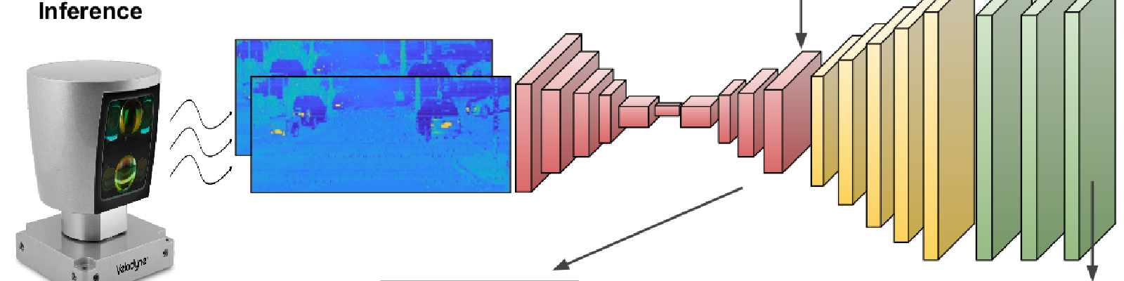
We introduce a deep architecture that given two consecutive low-resolution and sparse lidar scans, produces a high-resolution and dense optical flow, equivalent to one that would be computed from images. Our approach, therefore, can replace RGB cameras when the quality images is poor due to e.g. adverse weather conditions. Inference is done from only lidar scans.
Dense optical flow prediction from sparse lidar inputs only. Notice that the RGB images shown in the top-left are only considered to generate the pseudo ground-truth used during training.
Hallucinating Dense Optical Flow
Network Proposed
We propose a CNN architecture to hallucinate dense high resolution 2D optical flow in the image domain using as input only sparse and low resolution lidar information. Our network bridges the gap between lidar and camera domains, so that when the camera images are spoiled (e.g. at night sequences or due to heavy fog), we can still provide an accurate optical flow to directly substitute the degenerated image-based prediction in any vehicle navigation algorithm.
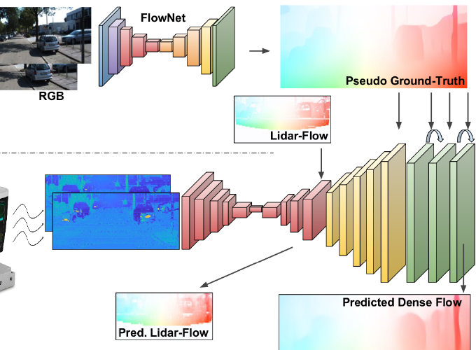
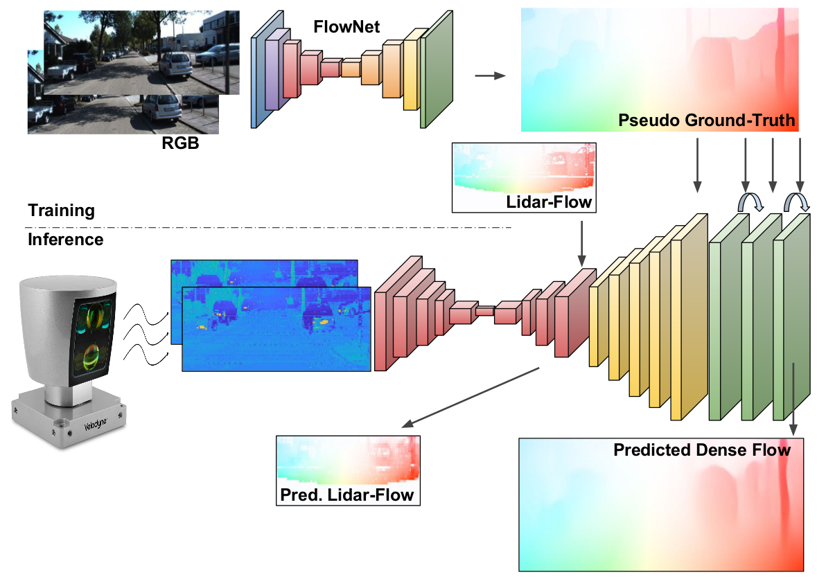
We have devised an elaborated architecture, consisting of three main blocks. The first one estimates the motion in the sparse lidar domain using a specific architecture resembling FlowNet, and it is trained with a ground-truth lidar optical flow obtained from RGB images. The second block performs the domain transformation and upsampling, guiding the learning towards predicting the final optical flow in the image domain. Finally, a refinement step is implemented to produce more accurate, dense, and visual appealing predictions.
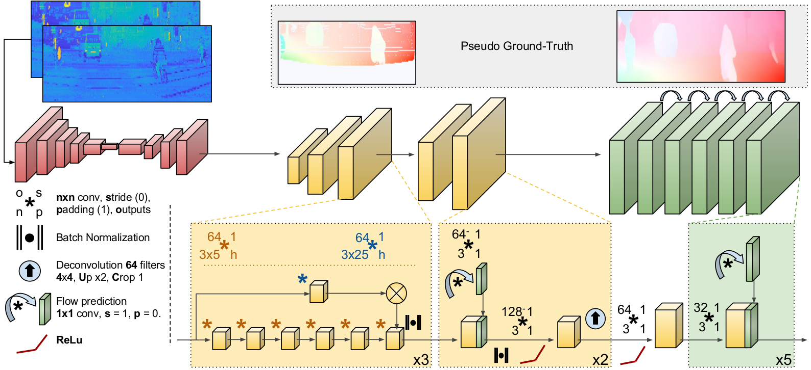
Lidar to dense optical-flow architecture. The proposed network is made of three main blocks sequentially connected which resolve the problem in different stages: 1) Estimation of the lidar-flow in low resolution (red layers); 2) Low-to-high resolution flow transformation and lidar-to-image domain change (yellow layers); 3) Final flow refinement (green layers).
Lidar-Flow
The first block of our proposed architecture aims at predicting \textit{lidar flow}, this is, the low resolution flow in the lidar domain from two consecutive lidar point clouds $\mathcal{X}_t$ and $\mathcal{X}_{t+1}$. The ground truth lidar flow for this problem, $GT_{Lidar}\in \mathbb{R}^{N \times M \times 2}$, is computed by projecting the lidar point cloud $\mathcal{X}_t$ onto the dense image flow $GT_{Dense}$ and keeping the motion and reflectance values of the overlapping points. Since the input lidar frames are low resolution, noisy and scattered, so will it be $GT_{Lidar}$.
In order to learn this low dimensional flow, we train a network $\mathcal{Y}_{Lidar} = \mathcal{G}_{\theta_{Lidar}}(\mathcal{X}_t, \mathcal{X}_{t+1}; \theta_{Lidar}; GT_{Lidar})$, being $\mathcal{Y}_{Lidar}$ the predicted lidar-flow and $\theta_{Lidar}$ the trainable parameters of the network $\mathcal{G}_{\theta_{Lidar}}$.
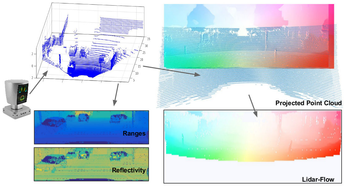
Building a lidar-to-optical flow dataset. Given a 3D point cloud from a laser scan (top-left) we create our input tensots with the range and reflectivity information (bottom-left) to be used as our inputs. Lidar-flow pseudo ground-truth is alsoe created by cropping the overlaping areas between the dense image-flow and the projected point cloud (bottom-right).
Lidar-to-Image Domain Transformation
The second major block of the proposed architecture is in charge of bringing the low resolution lidar flow to the high resolution image domain. Specifically, this block receives as input the lidar flow $\mathcal{Y}_{Lidar}$ predictions along with the accordingly downscaled input lidar frames and produces as output an upscaled image-centered optical flow prediction learned from $GT_{Dense}$. This upscaling operation can be formally written as $\mathcal{Y}_{Up} = \mathcal{H}_{\theta_{Up}}(\mathcal{X}^{\prime}_{t}, \mathcal{X}^{\prime}_{t+1}, \mathcal{Y}_{Lidar}; \theta_{Up}; GT_{Dense})$, where $\mathcal{H}_{\theta_{Up}}$ represents the model with learned parameters $\theta_{Up}$, $\mathcal{X}^{\prime}$ refers to the 1⁄2 downsampled input lidar frames that match the $\mathcal{Y}_{Lidar}$ resolution, and $\mathcal{Y}_{Up} \in \mathbb{R}^{H \times W \times 2}$ is the output predicted optical flow in the image domain.
In order to actively guide this domain transformation process, we devise an architecture with two sub-blocks (shown in yellow in the network Figure). The first sub-block consists of a set of multi-scale filters in two convolutional branches, providing context knowledge to the network. In one branch we produce high frequency features by applying $5$ consecutive convolutional layers with small $3 \times 5$ filters and without any lateral padding (which allows the feature maps to grow horizontally for matching the desired output resolution). In the other branch, lower frequency features are generated with a convolution layer using wider $3 \times 25$ filters and outputting the same feature map resolution. Finally, the features of the two branches are concatenated.
Hallucinated Optical Flow Refinement
We design a similar iterative convolutional approach for refining the hallucinated optical flow prediction, as is sketched in the green block of the network figure, so that avoiding the computational burden of a CRF and obtaining a fully end-to-end procedure.
We formally denote this final refinement step as $\mathcal{Y}_{End} = \mathcal{K}_{\theta_{End}}(\mathcal{Y}_{Up}; \theta_{End}; GT_{Dense})$. It works by performing a prediction of the final optical flow, which is concatenated to the feature maps of the previous convolutional layer. The concatenated tensor is then passed to another block that generates again new feature maps and a new optical flow prediction, but this time with a better knowledge of the desired output. As shown in the green block of the network figure, this process is repeated 5 times, simulating an iterative scheme.
Results
Qualitative Results

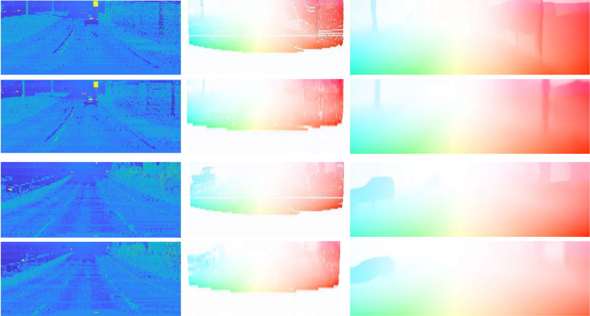
Qualitative results of the presented system.
All images are taken during inference from our validation lidar-image-flow set, so none of them were previously seen during training. We show four different example scenes, grouped in 4 quadrants. In each quadrant there are three columns, representing the following. Column 1: lidar inputs $X$ t and $X_{t+1}$ ; Column 2-top: lidar flow pseudo ground-truth $GT_{Lidar}$ ; Column 2-bottom: lidar flow prediction $Y_{Lidar}$ ; Column 3-top: dense pseudo ground-truth, GT Dense ; Column 3-bottom: final predicted dense optical flow $Y_{End}$.
Quantitative Results
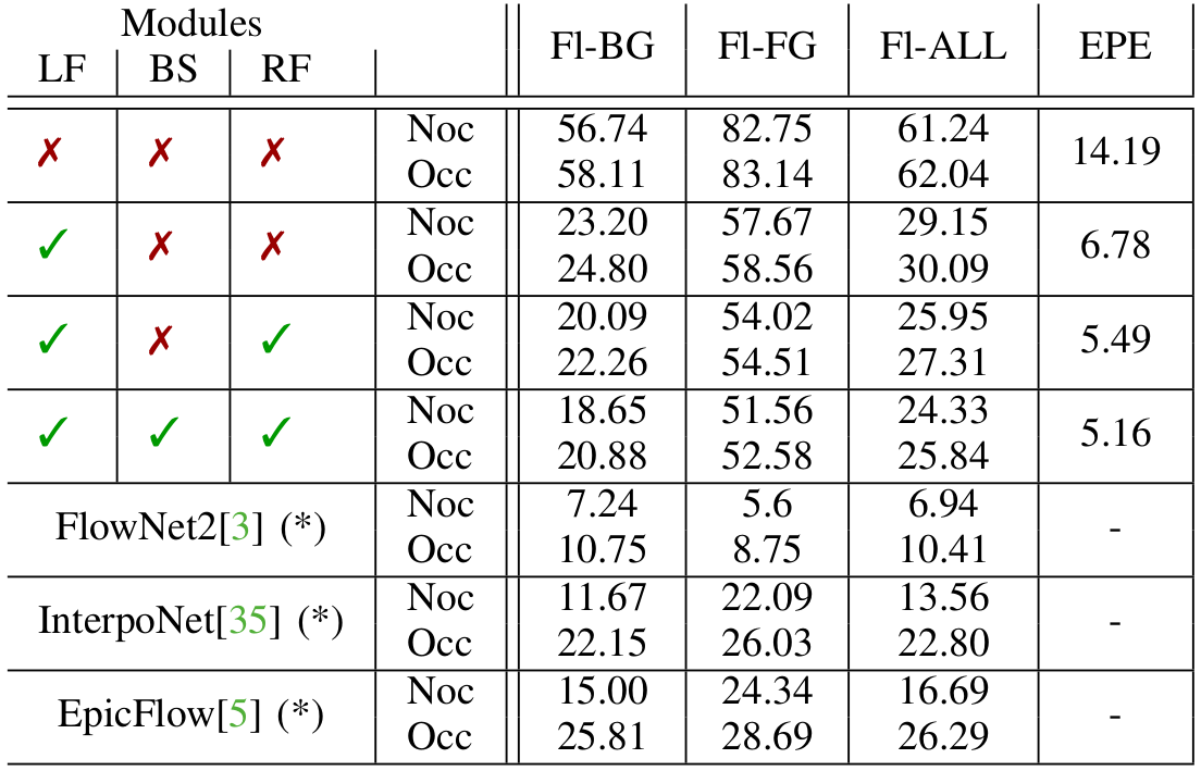
Quantitative evaluation and comparison with image-based optical-flow methods. (*) indicates that for these methods the test set is slightly bigger from the one used for our approach, as we could no obtain all the corresponding lidar frames.
Flow for background, foreground and all is measured for both non-occluded and full points, as in the Kitti Flow benchmark. The End-Point-Error (EPE) is measured against the pseudo ground-truth computed using FlowNet2. Although indicative, these results show that our lidar-based approach is on par with other well-known optical flow algorithms that rely on higher resolution and quality input images.
Acknowledgements: This work has been supported by the Spanish Ministry of Economy, Industry and Competitiveness projects COLROBTRANSP (DPI2016-78957-R), HuMoUR (TIN2017-90086-R), the Spanish State Research Agency through the Maria de Maeztu Seal of Excellence (MDM-2016- 0656), and the EU project LOGIMATIC (H2020-Galileo- 2015-1-687534). We also thank Nvidia for hardware donation under the GPU Grant Program.